NBA Scoring Options
Yahoo DFS Bankroll Analysis
Background
In the Tool section is a basic bankroll analysis tool for Yahoo Daily Fantasy Sports built on RStudio’s Shiny framework. The purpose of the tool is to provide basic information to help users make more informed decisions with their bankroll.
Below is a chart of my NFL Yahoo DFS history over the past year:
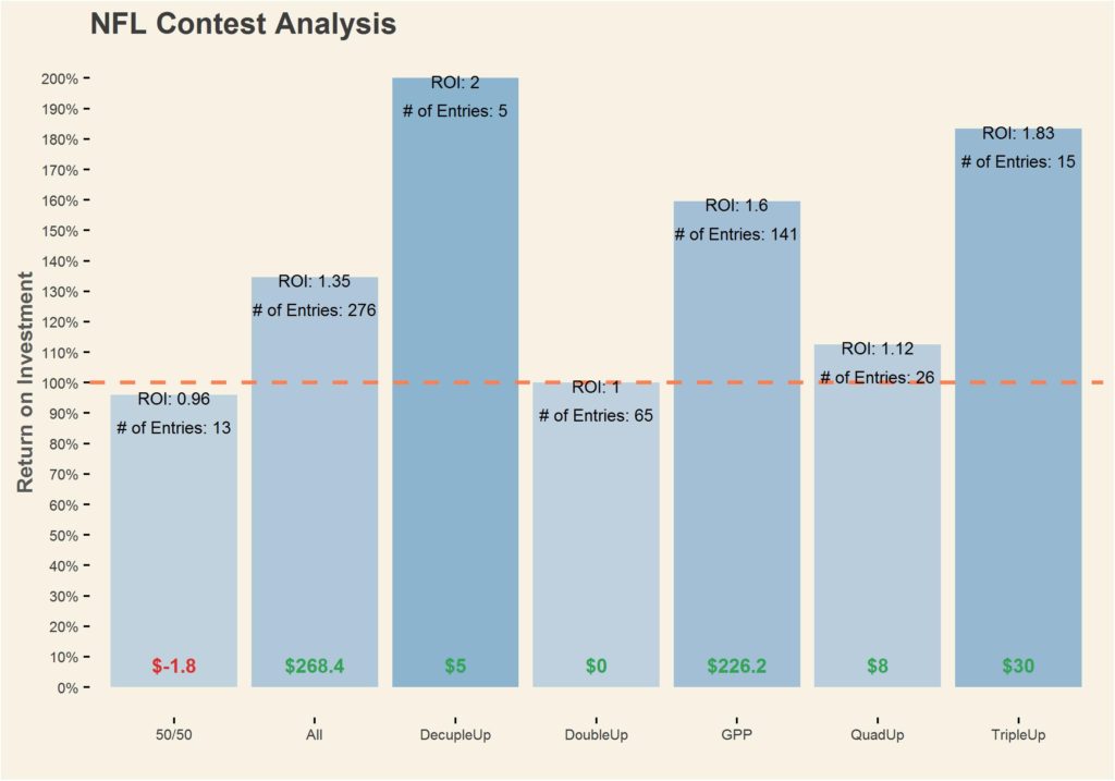
The above chart suggests that GPP & Quad Ups are the most successful, while Double Ups have been less successful (ROI = 1 indicates break even). Decuple Ups and Triple Ups show promise, but with a low amount of contests played, it’s difficult to determine the efficacy of each chart.
Tool
The Riddler – Will You (Yes, You) Decide The Election?
Twice is always nice, so I’m going to tackle the Classic Riddler for the week as well.
For those that aren’t familiar, The Riddler is a weekly puzzle series from Oliver Roeder at FiveThirtyEight that usually involves some combination of math, logic and probability.
This weeks Riddler Classic is:
You are the only sane voter in a state with two candidates running for Senate. There are N other people in the state, and each of them votes completely randomly! Those voters all act independently and have a 50–50 chance of voting for either candidate. What are the odds that your vote changes the outcome of the election toward your preferred candidate?
More importantly, how do these odds scale with the number of people in the state? For example, if twice as many people lived in the state, how much would your chances of swinging the election change?
As with most other Riddler problems, I want to start with doing some of the basic cases when N is low. As per our friend at 538, Ollie, we’ll deal with ties as such:
@ianrhile assume a coin flip if you’d like. or just assume an odd number of voters.
— Oliver Roeder (@ollie) November 4, 2016
So let’s start with the basic case of N=1 (1 other voter). The voter can either vote for your preferred candidate (D) or your non-preferred candidate ®. You’ll always be voting for your preferred candidate (D). Our goal is to find out what percent of the time that will make a difference. So let’s take a look at the scenarios that could happen:
| Scenario | Votes D | Votes R | Chance of Scenario |
| A | 1 | 0 | 0.5 |
| B | 0 | 1 | 0.5 |
Pretty simple. In Scenario A, your candidate’s winning, so your vote for candidate D doesn’t matter. If Scenario B happens, you can force a tie, which according to Ollie goes to a coin flip. So the probability of you affecting the election (P1) is:
P1 = (Probability of Scenario B)*(Probability that Tiebreaker Coinflip Lands in Your Favor)
P1 = 0.5 *0.5 = 0.25
Simple enough, let’s look at P2. The voters here can either go DD (both vote for D), RR, DR, or RD. Since the last two states are the same for our purposes, we can sum up the system at N=2 as:
| Scenario | Votes D | Votes R | Chance of Scenario |
| A | 2 | 0 | 0.25 |
| B | 0 | 2 | 0.25 |
| C | 1 | 1 | 0.5 |
In Scenario A , your candidate won, so it doesn’t really matter to us. In Scenario B, your 1 vote for Candidate D won’t influence the result so that’s not relevant either. So we look at Scenario C, however there’s no coinflip element here therefore:
P2 = Probability of Scenario C = 0.5
Let’s jump ahead to N=5 so we can deal with a more interesting scenario. The states that can exist at N=5 are:
| Scenario | Votes D | Votes R | Chance of Scenario |
| A | 0 | 5 | 0.03125 |
| B | 1 | 4 | 0.15625 |
| C | 2 | 3 | 0.3125 |
| D | 3 | 2 | 0.3125 |
| E | 4 | 1 | 0.15625 |
| F | 5 | 0 | 0.03125 |
There’s two important things to notice here. There’s really only one scenario where we can affect the result in our favor (Scenario C, where we can force a tie). By now we see a pattern in the types of scenarios that our vote can influence — we can either force a tie as shown in Scenario C for N=5 or break a tie as shown in Scenario C for N =3 earlier. Those situations can be defined as:
Situations Where Our Vote Matters = [N/2]
The nearest integer function (as denoted by [x]) rounds down a number to nearest integer (e.g. [2.5] = 2). Cool, now we know for a given N which scenarios we can actually influence.
Before N=5, calculating the probability was rather trivial. For larger N we can fall back on the Binomial Probability Formula defined by:
Pk successes in n trials = nCr(n,k)*pk*(1‑p)n‑k
Each of those terms are:
nCr(n,k) = Amount of unordered combinations for a given k objects in set of n total objects (e.g. how many unique ways can you have 2 heads given 5 coins). Defined by n!/((n‑k)!*k!).
k = Successes. For our problem, that’ll be votes cast for Candidate D
p = Probability of success
Since we’re dealing with 50/50 odds, a lot of that formula can get simplified. Also, we defined the scenarios that we can affect as ones where Canidate D votes = [N/2], therefore k = [N/2]. That results in the simplified formula:
Pk successes in n trials = nCr(n,k)*pk*(1‑p)n‑k = nCr(n,k)*0.5k*(0.5)n‑k = nCr(n,k)*0.5k+n‑k = nCr(n,k)*0.5n = nCr(n,[n])*0.5n
PScenario our vote counts @ given N = N!/((N-[N/2])!*[N/2]!)*0.5N
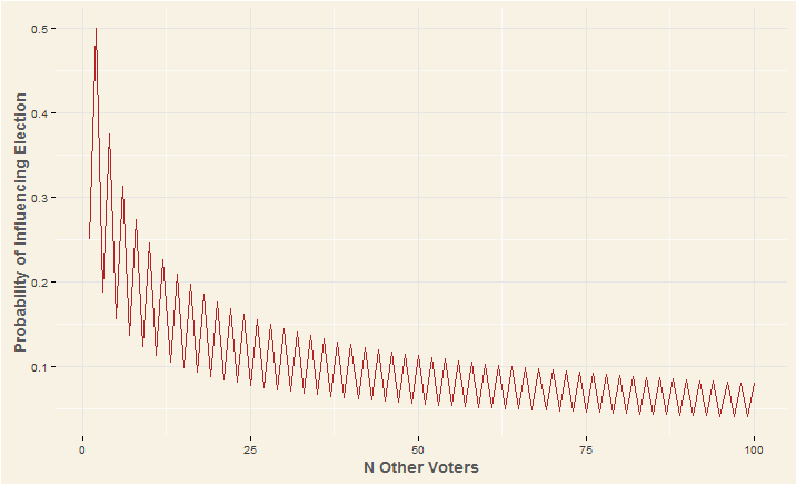
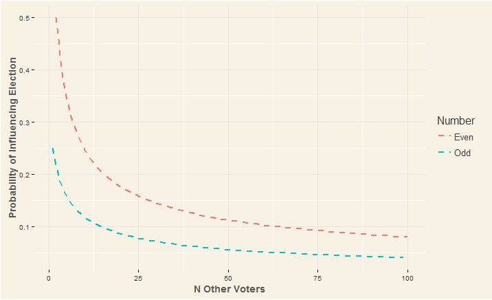
Recall that at odd N’s our vote just forced a tie in this scenario, and we had to account for . So in actuality, the general solution is a bit disjointed. The solution is:
For Even N
PEven N = N!/((N-[N/2])!*[N/2]!)*0.5N
For Odd N
POdd N = 0.5*N!/((N-[N/2])!*[N/2]!)*0.5N
This relationship can be described in the following graphs:
The Riddler – Alligators, Sharks, Bridges and Friends

It’s been a very long time since I’ve updated this, and while some if it has been laziness on my part, most of the blame can be blamed on Northwestern EDI — an awesome Master’s program I started about 2 months ago (also the last time I posted an update). It’s been a great experience so far, and the program’s going to be the catalyst for a lot of the work I’ll be posting from here on out.
Without further ado, The Riddler [Express].
For those that aren’t familiar, The Riddler is a weekly puzzle series from Oliver Roeder at FiveThirtyEight that usually involves some combination of math, logic and probability. The Riddler Express is a simpler version of the classic Riddler.
Four people have to cross an old, rickety bridge over deep, cold water infested with sharks, alligators, crocodiles and shrieking eels. The bridge is so old that it can hold no more than two people at any given time. It’s the middle of the night, so on every trip across the bridge, the person crossing needs to use the group’s only flashlight to cross safely. The four people who need to cross all walk at different speeds. One of them takes one minute to cross, one takes two minutes, one takes five minutes and one takes 10 minutes. If two people cross together, they need to stay together to share the flashlight, so they cross at the speed of the slower person. For example, the one-minute person can cross with the 10-minute person, and that trip would take 10 minutes.
How quickly can all four people get across the bridge?
So your first thought, as mine was, might have been to include the 1 Minute man (hereby referred to as 1M) in every transaction. That gives us a solution in 19 minutes (as illustrated by the gif below!).
 1
1
If my excellent artwork didn’t make sense, here’s a table explaining what happened.
| Side A | Side B | Time Elapsed |
| 1M, 2M, 5M, 10M | X | 0 Minutes |
| 5M, 10M | 1M, 2M | 2 Minutes |
| 1M, 5M, 10M | 2M | 3 Minutes |
| 10M | 1M, 2M, 5M | 8 Minutes |
| 1M, 10M | 2M, 5M | 9 Minutes |
| X | 1M, 2M, 5M, 10M | 19 Minutes |
So that gets us at a modest 19 minutes, but actually we can do better. Instead of making 1M run all over the place, we’re going to give him a break on Side B. The issue with the above solution is that we’re wasting a total of 15 minute getting 10M and 5M across. Ideally, you’d like 10M and 5M to go across together to mitigate the lost time, but still make it so that one of them doesn’t have to walk back.
The below gif illustrates the optimal solution of 17 minutes.

Again, if that didn’t make sense here’s a table:
| Side A | Side B | Time Elapsed |
| 1M, 2M, 5M, 10M | X | 0 Minutes |
| 5M, 10M | 1M, 2M | 2 Minutes |
| 1M, 5M, 10M | 2M | 3 Minutes |
| 1M | 2M, 5M, 10M | 13 Minutes |
| 1M, 2M | 5M, 10M | 15 Minutes |
| X | 1M, 2M, 5M, 10M | 17 Minutes |
You can see here that we were able to save time by making 5M & 10M go over together without making one of them walk back, giving the optimal solution of 17 minutes.
The Riddler — How Many Bananas Does It Take To Lead A Camel To Market?
Took along hiatus from the Riddler, but I’m back!
For those that aren’t familiar, The Riddler is a weekly puzzle series from Oliver Roeder at FiveThirtyEight that usually involves some combination of math, logic and probability.
This weeks FiveThirtyEight Riddler, How Many Bananas Does it Take to Lead a Camel to Market?:
sYou have a camel and 3,000 bananas. (Because of course you do.) You would like to sell your bananas at the bazaar 1,000 miles away. Your loyal camel can carry at most 1,000 bananas at a time. However, it has an insatiable appetite and quite the nose for bananas — if you have bananas with you, it will demand one banana per mile traveled. In the absence of bananas on his back, it will happily walk as far as needed to get more bananas, loyal beast that it is. What should you do to get the largest number of bananas to the bazaar? What is that number?
So just in order to get to the market, you need a minimum of 1,000 bananas, and since that just gets you there without any bananas to sell, a more creative solution is required. Let’s say we split the 3,000 bananas into 3 piles — Pile A, Pile B, & Pile C. From there we move Pile A one mile, go back and do the same for Piles B & C.
| Mile | Pile A | Pile B | Pile C |
|---|---|---|---|
| 0 | 1000 | 1000 | 1000 |
| 1 | 999 | 999 | 999 |
This won’t get us anywhere, since at mile 1,000 we’ll be left with 0 bananas in each. Let’s instead redistribute the Pile C bananas to Pile A and Pile B.
| Mile | Pile A | Pile B | Pile C |
|---|---|---|---|
| 0 | 1000 | 1000 | 1000 |
| 1 | 999 | 999 | 999 |
| 1 | 1000 | 1000 | 997 |
Now if we were to just move each pile forward without redistribution we’d end up with 2 bananas to sell at the market (1 from Pile A and 1 from Pile B). Let’s redistribute the bananas every mile, now it looks like:
| Mile | Pile A | Pile B | Pile C |
|---|---|---|---|
| 0 | 1000 | 1000 | 1000 |
| 1 | 999 | 999 | 999 |
| 1 | 1000 | 1000 | 997 |
| 2 | 999 | 999 | 996 |
| 2 | 1000 | 1000 | 995 |
| 3 | 999 | 999 | 994 |
| 3 | 1000 | 1000 | 992 |
A pattern starts to emerge, every mile takes 3 bananas, specifically from Pile C. For now, let’s say:
Bananas in Pile C = 1000 — 3*Miles Traveled
Now let’s look at Mile 333, about when Pile C would be exhausted.
| Mile | Pile A | Pile B | Pile C |
|---|---|---|---|
| 333 | 1000 | 1000 | 1 |
| 334 | 999 | 999 | 0 |
Since we only have 1 banana left in Pile C, we can’t redistribute it. So we’re now 667 miles away from our destination, with 2 piles of 1,000 bananas each. Let’s continue this redistribution strategy with Piles A and Pile B (redistributing Pile B)
| Mile | Pile A | Pile B | Pile C |
|---|---|---|---|
| 334 | 999 | 999 | 0 |
| 334 | 1000 | 998 | 0 |
| 335 | 999 | 997 | 0 |
| 335 | 1000 | 995 | 0 |
Now another pattern emerges for Pile B. The amount of bananas in Pile B can be described as:
Bananas in Pile B = 1000 — 2*(Miles Traveled-333)
Using this we see that Pile B runs out bananas around mile 833.
| Mile | Pile A | Pile B | Pile C |
|---|---|---|---|
| 832 | 1000 | 2 | 0 |
| 833 | 999 | 1 | 0 |
| 833 | 1000 | 0 | 0 |
At this point, we can simply just carry Pile A, feeding a banana to the camel every mile for the last 177 miles. The amount of bananas left when we reach the market is simply 1000 — 177 = 833.
To answer the original Riddler question, the largest amount of bananas that we can get to the bazaar under the current circumstances is 833.
Project — Robot Design

Nylon Calculus — Age and upside in the NBA Draft
Kaggle — Integer Sequence Learning

Project Focus:
Data Science • R
Project Overview
As both a hobby and to better my data science skills, I compete in Kaggle’s Data Science competitions. This particular competition stands out as it forced me to critically examine the methods I was using, and because I ended up peaking at number 2 on the leaderboard (finally finishing in the 31st, 89th percentile).
Skills Used
The crux of the script was a combination of simpler sequence guessing models (mode & frequency) and a more robust tuning model. The difficulty was in tuning the script to select the correct model (mode, frequency or linear regression) to solve a sequence.
Project
I recently submitted an entry into Kaggle’s Integer Sequence Learning Competition, and as of right now, it’s 2nd on the leaderboard. I wanted to go over my methodology, and how I got to my submission.
The Competition
For the competition, we’re asked to predict the last term of a sequence. The description given by the competition:
7. You read that correctly. That’s the start to a real integer sequence, the powers of primes. Want something easier? How about the next number in 0, 1, 1, 2, 3, 5, 8, 13, 21, 34, 55? If you answered 89, you may enjoy this challenge. Your computer may find it considerably less enjoyable.
The On-Line Encyclopedia of Integer Sequences is a 50+ year effort by mathematicians the world over to catalog sequences of integers. If it has a pattern, it’s probably in the OEIS, and probably described with amazing detail. This competition challenges you create a machine learning algorithm capable of guessing the next number in an integer sequence. While this sounds like pattern recognition in its most basic form, a quick look at the data will convince you this is anything but basic!
The Methodology
The sequences are made up of a linear sequences, logarithmic sequences, sequences with a modulus, and many other oddities. In the below graph, generated through this script by Kaggle User Calin Uioreanu, illustrates some of these sequences and gives an idea of what we’re working with.

Now that we have a better idea of what we’re working with, lets get into the methodology.
We’re given 3 files to start:
- train.csv
- test.csv
- sample_submission.csv
All fairly normal as far as Kaggle competitions go. I won’t be using the training data, and will be jumping straight into the test data.
library(plyr)
library(dplyr)
library(readr)
library(stringr)
options(scipen=999) #Prevents Scientific Notation for Large Numbers
Here I’m just loading the necessary libaries we’ll need for the code. Note the “options(scipen=999),” that’s important to prevent R from formatting the larger numbers into scientific notation.
Also note that reading test.csv produces a data frame of two variables, Id and Sequence. The Id variables are integers, and are exactly how we want them. The Sequence variable is in strings, so we’ll need to convert that to a list a of numbers. It’s a pretty simple use of the str_split() function; I particularly liked how Kaggle User William Cukierski wrote his method, so I implemented that in my code as well.
parseSequence <- function(str) {
  return(as.numeric(str_split(str, ",")[[1]]))
}
So now into how we’re actually going to predict what the last term of each sequence is. That’ll be done using the following 3 methods in this order (i.e. if method 1 fails, move onto method 2):
- Linear Fit
- Frequency Table
- Mode
Let’s start with the Mode methodology since it’s the simplest. For this, you simply find the mode in a given sequence, and that’ll be your guess for the last term in the sequence. The Mode Benchmark seen on the Leaderboard has an accuracy of 5.7%, so it’s a decent fall-back if our first two options fail.
Mode <- function(x) {
  ux <- unique(x)
  ux[which.max(tabulate(match(x, ux)))]
}
A lot of these sequences are sub-sequences of other sequences within our dataset. So we’ll be looking at the last term in each sequence (i.e. say a sequence ends 185), find other sequences that contain that number (i.e. say 10 sequences contain 185), and then find what follows that number (i.e. if 287 follows 185 in 7/10 sequences, that’ll be our guess). This idea was inspired by this script on Kaggle
buildFrequencyTable <- function(sequences)
{
  # Collate all pairs of consecutive integers across all sequences
  pairs <- ldply(sequences,
                 function(sequence)
                 {
                   if(length(sequence) <= 2)
                   {
                     return(NULL)
                   }
                   data.frame(last=head(sequence,-1),
                              following=tail(sequence,-1))
                 })

  # For each unique integer across all sequences, find the most common
  # integer that comes next
  frequencyTable <- ddply(pairs,
                          "last",
                          function(x)
                          {
                            data.frame(last=x$last[1],
                                       following=Mode(x$following))
                          })

  return(frequencyTable)
}
That’s the method itself. It’ll generate a Frequency Table that lists the integer most commonly following every unique integer. To integrate into code simply:
test<-read.csv("test.csv")
test$Sequence<- sapply(test$Sequence, FUN = parseSequence)
frequencyTable <- buildFrequencyTable(test$Sequence)
test$last <- sapply(test.sample$Sequence,
                           function(sequence) tail(unlist(sequence),1))
test <- join(test,frequencyTable,type="left")
This gives a a data frame, test, with 4 variables — Id (ID variable), Sequence (the sequence), last (the last term in the sequence) & following (the most common integer following the last term in the sequence). We’ll be using this in our Linear Fit Prediction.
The Linear Fit prediction code is below
predictor<-function(seq.data,freq.soln){
  seq<-unlist(seq.data)
  if(length(seq)<2){
    return(tail(seq,1))
  }

  for(numberOfPoints in 1:(length(seq)-1)){
    df <- data.frame(y=tail(seq,-numberOfPoints))

    formulaString <- "y~"

    for(i in 1:(numberOfPoints))
    {
      df[[paste0("x",i)]] <- seq[i:(length(seq)-numberOfPoints+i-1)]
      formulaString <- paste0(formulaString,"+x",i)
    }

    fit <- lm(formula(formulaString),df)
    mae <- max(abs(fit$residuals))

    df <- list()
    for(i in 1:numberOfPoints)
    {
      df[[paste0("x",i)]] <- seq[length(seq)-numberOfPoints+i]
    }
    prediction<-predict(fit,df) if(mae>0 && mae<1){
      return(round(prediction))
    }
  }
  if(!is.na(freq.soln)){
    return(freq.soln)
  }


    return(Mode(seq))

}
I’ll break down the individual components of that code block.
Here all we’re doing is unlisting the sequence that came in so we can with it. The first check is to see if the sequence is just one integer — if so, we obviously can’t do anything with it and return the first element. I suppose this could be integrated into the Mode fallback, but if in the future I want to track how many short sequences there are, it helps.
  seq<-unlist(seq.data)
  iterations<<-iterations+1
  if(length(seq)<2){
    print("Returned Short Seq")
    return(tail(seq,1))
  }
  }
The linear model works backwards from a sequence. I got the inspiration (and most of the code) for this section from this script. The last X terms (defined by numberOfPoints) from the end of the sequence are used to model the sequence. The first for loop within the overarching for loop is used to create the formula string (i.e. y ~ x1 + x2 + x3…) that’ll be plugged into the linear model function, lm(). We also calculated what the maximum residual is.
Now that we have our model, we create a data frame of the values we need to use the predict() function and generate our prediction. To save some computation time, this code block cna be placed in the following if statement.
Recall the maximum residual we calculated earlier. If that value is 0, we likely have 0 degrees of freedom (more predictor variables than samples). This Stack Overflow post goes into it nicely. I used a maximum residual of less than 1 as a cut-off point to determine if a model was good enough. That can (& should be tuned) for maximum accuracy. If the linear model we’ve made for a given sequence meets that criteria we return the prediction from the linear fit.
  for(numberOfPoints in 1:(length(seq)-1)){
    df <- data.frame(y=tail(seq,-numberOfPoints))

    formulaString <- "y~"

    for(i in 1:(numberOfPoints))
    {
      df[[paste0("x",i)]] <- seq[i:(length(seq)-numberOfPoints+i-1)]
      formulaString <- paste0(formulaString,"+x",i)
    }

    fit <- lm(formula(formulaString),df)
    mae <- max(abs(fit$residuals))

    df <- list()
    for(i in 1:numberOfPoints)
    {
      df[[paste0("x",i)]] <- seq[length(seq)-numberOfPoints+i]
    }
    prediction<-predict(fit,df) if(mae>0 && mae<1){
      return(round(prediction))
    }
  }
If our linear model does not meet the criteria, we move on to our Frequent Solution method, and if that fails, Mode is the fail-safe.
 if(!is.na(freq.soln)){
    return(freq.soln)
  }

    return(Mode(seq))
To get the actual solution file out it’s simply:
results<-mapply(test.sample$Sequence, test.sample$following, FUN=predictor)
solution.df<-data.frame(test.sample$Id,results)
colnames(solution.df)<-c('Id','Last')
write.csv(solution.df,file="Soln.csv",row.names = F)
This yields a solution that’s 18.63% accurate, good for 2nd on the leaderboard as of June 20th. I’d like to acknowledge the following scripts:
Those scripts did the brunt of the work, and taught me a lot. I highly recommend them.
The Methodology
Obviously there’s a lot that can still be added to this script. Currently ~27% of predictions use the linear model, ~38% use frequency prediction and ~34% use the mode prediction. Looking through some of the sequences by hand, this model misses on a lot of geometric sequences and sequences with a modulus term. I’m not entirely sure to attack sequences with a modular term, but I’d imagine sequences with a geometric term can be modeled. The immediate next step is to add an additional model between the linear model and frequency model step. hopefully lowering the amount of sequences that require the Mode fallback.