Project Focus:
Data Science • R
Project Overview
As both a hobby and to better my data science skills, I compete in Kaggle’s Data Science competitions. This particular competition stands out as it forced me to critically examine the methods I was using, and because I ended up peaking at number 2 on the leaderboard (finally finishing in the 31st, 89th percentile).
Skills Used
The crux of the script was a combination of simpler sequence guessing models (mode & frequency) and a more robust tuning model. The difficulty was in tuning the script to select the correct model (mode, frequency or linear regression) to solve a sequence.
Project
I recently submitted an entry into Kaggle’s Integer Sequence Learning Competition, and as of right now, it’s 2nd on the leaderboard. I wanted to go over my methodology, and how I got to my submission.
The Competition
For the competition, we’re asked to predict the last term of a sequence. The description given by the competition:
7. You read that correctly. That’s the start to a real integer sequence, the powers of primes. Want something easier? How about the next number in 0, 1, 1, 2, 3, 5, 8, 13, 21, 34, 55? If you answered 89, you may enjoy this challenge. Your computer may find it considerably less enjoyable.
The On-Line Encyclopedia of Integer Sequences is a 50+ year effort by mathematicians the world over to catalog sequences of integers. If it has a pattern, it’s probably in the OEIS, and probably described with amazing detail. This competition challenges you create a machine learning algorithm capable of guessing the next number in an integer sequence. While this sounds like pattern recognition in its most basic form, a quick look at the data will convince you this is anything but basic!
The Methodology
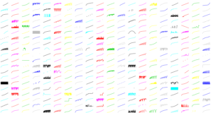
The sequences are made up of a linear sequences, logarithmic sequences, sequences with a modulus, and many other oddities. In the below graph, generated through this script by Kaggle User Calin Uioreanu, illustrates some of these sequences and gives an idea of what we’re working with.

Now that we have a better idea of what we’re working with, lets get into the methodology.
We’re given 3 files to start:
- train.csv
- test.csv
- sample_submission.csv
All fairly normal as far as Kaggle competitions go. I won’t be using the training data, and will be jumping straight into the test data.
library(plyr)
library(dplyr)
library(readr)
library(stringr)
options(scipen=999) #Prevents Scientific Notation for Large Numbers
Here I’m just loading the necessary libaries we’ll need for the code. Note the “options(scipen=999),” that’s important to prevent R from formatting the larger numbers into scientific notation.
Also note that reading test.csv produces a data frame of two variables, Id and Sequence. The Id variables are integers, and are exactly how we want them. The Sequence variable is in strings, so we’ll need to convert that to a list a of numbers. It’s a pretty simple use of the str_split() function; I particularly liked how Kaggle User William Cukierski wrote his method, so I implemented that in my code as well.
parseSequence <- function(str) {
  return(as.numeric(str_split(str, ",")[[1]]))
}
So now into how we’re actually going to predict what the last term of each sequence is. That’ll be done using the following 3 methods in this order (i.e. if method 1 fails, move onto method 2):
- Linear Fit
- Frequency Table
- Mode
Let’s start with the Mode methodology since it’s the simplest. For this, you simply find the mode in a given sequence, and that’ll be your guess for the last term in the sequence. The Mode Benchmark seen on the Leaderboard has an accuracy of 5.7%, so it’s a decent fall-back if our first two options fail.
Mode <- function(x) {
  ux <- unique(x)
  ux[which.max(tabulate(match(x, ux)))]
}
A lot of these sequences are sub-sequences of other sequences within our dataset. So we’ll be looking at the last term in each sequence (i.e. say a sequence ends 185), find other sequences that contain that number (i.e. say 10 sequences contain 185), and then find what follows that number (i.e. if 287 follows 185 in 7/10 sequences, that’ll be our guess). This idea was inspired by this script on Kaggle
buildFrequencyTable <- function(sequences)
{
  # Collate all pairs of consecutive integers across all sequences
  pairs <- ldply(sequences,
                 function(sequence)
                 {
                   if(length(sequence) <= 2)
                   {
                     return(NULL)
                   }
                   data.frame(last=head(sequence,-1),
                              following=tail(sequence,-1))
                 })

  # For each unique integer across all sequences, find the most common
  # integer that comes next
  frequencyTable <- ddply(pairs,
                          "last",
                          function(x)
                          {
                            data.frame(last=x$last[1],
                                       following=Mode(x$following))
                          })

  return(frequencyTable)
}
That’s the method itself. It’ll generate a Frequency Table that lists the integer most commonly following every unique integer. To integrate into code simply:
test<-read.csv("test.csv")
test$Sequence<- sapply(test$Sequence, FUN = parseSequence)
frequencyTable <- buildFrequencyTable(test$Sequence)
test$last <- sapply(test.sample$Sequence,
                           function(sequence) tail(unlist(sequence),1))
test <- join(test,frequencyTable,type="left")
This gives a a data frame, test, with 4 variables — Id (ID variable), Sequence (the sequence), last (the last term in the sequence) & following (the most common integer following the last term in the sequence). We’ll be using this in our Linear Fit Prediction.
The Linear Fit prediction code is below
predictor<-function(seq.data,freq.soln){
  seq<-unlist(seq.data)
  if(length(seq)<2){
    return(tail(seq,1))
  }

  for(numberOfPoints in 1:(length(seq)-1)){
    df <- data.frame(y=tail(seq,-numberOfPoints))

    formulaString <- "y~"

    for(i in 1:(numberOfPoints))
    {
      df[[paste0("x",i)]] <- seq[i:(length(seq)-numberOfPoints+i-1)]
      formulaString <- paste0(formulaString,"+x",i)
    }

    fit <- lm(formula(formulaString),df)
    mae <- max(abs(fit$residuals))

    df <- list()
    for(i in 1:numberOfPoints)
    {
      df[[paste0("x",i)]] <- seq[length(seq)-numberOfPoints+i]
    }
    prediction<-predict(fit,df) if(mae>0 && mae<1){
      return(round(prediction))
    }
  }
  if(!is.na(freq.soln)){
    return(freq.soln)
  }


    return(Mode(seq))

}
I’ll break down the individual components of that code block.
Here all we’re doing is unlisting the sequence that came in so we can with it. The first check is to see if the sequence is just one integer — if so, we obviously can’t do anything with it and return the first element. I suppose this could be integrated into the Mode fallback, but if in the future I want to track how many short sequences there are, it helps.
  seq<-unlist(seq.data)
  iterations<<-iterations+1
  if(length(seq)<2){
    print("Returned Short Seq")
    return(tail(seq,1))
  }
  }
The linear model works backwards from a sequence. I got the inspiration (and most of the code) for this section from this script. The last X terms (defined by numberOfPoints) from the end of the sequence are used to model the sequence. The first for loop within the overarching for loop is used to create the formula string (i.e. y ~ x1 + x2 + x3…) that’ll be plugged into the linear model function, lm(). We also calculated what the maximum residual is.
Now that we have our model, we create a data frame of the values we need to use the predict() function and generate our prediction. To save some computation time, this code block cna be placed in the following if statement.
Recall the maximum residual we calculated earlier. If that value is 0, we likely have 0 degrees of freedom (more predictor variables than samples). This Stack Overflow post goes into it nicely. I used a maximum residual of less than 1 as a cut-off point to determine if a model was good enough. That can (& should be tuned) for maximum accuracy. If the linear model we’ve made for a given sequence meets that criteria we return the prediction from the linear fit.
  for(numberOfPoints in 1:(length(seq)-1)){
    df <- data.frame(y=tail(seq,-numberOfPoints))

    formulaString <- "y~"

    for(i in 1:(numberOfPoints))
    {
      df[[paste0("x",i)]] <- seq[i:(length(seq)-numberOfPoints+i-1)]
      formulaString <- paste0(formulaString,"+x",i)
    }

    fit <- lm(formula(formulaString),df)
    mae <- max(abs(fit$residuals))

    df <- list()
    for(i in 1:numberOfPoints)
    {
      df[[paste0("x",i)]] <- seq[length(seq)-numberOfPoints+i]
    }
    prediction<-predict(fit,df) if(mae>0 && mae<1){
      return(round(prediction))
    }
  }
If our linear model does not meet the criteria, we move on to our Frequent Solution method, and if that fails, Mode is the fail-safe.
 if(!is.na(freq.soln)){
    return(freq.soln)
  }

    return(Mode(seq))
To get the actual solution file out it’s simply:
results<-mapply(test.sample$Sequence, test.sample$following, FUN=predictor)
solution.df<-data.frame(test.sample$Id,results)
colnames(solution.df)<-c('Id','Last')
write.csv(solution.df,file="Soln.csv",row.names = F)
This yields a solution that’s 18.63% accurate, good for 2nd on the leaderboard as of June 20th. I’d like to acknowledge the following scripts:
Those scripts did the brunt of the work, and taught me a lot. I highly recommend them.
The Methodology
Obviously there’s a lot that can still be added to this script. Currently ~27% of predictions use the linear model, ~38% use frequency prediction and ~34% use the mode prediction. Looking through some of the sequences by hand, this model misses on a lot of geometric sequences and sequences with a modulus term. I’m not entirely sure to attack sequences with a modular term, but I’d imagine sequences with a geometric term can be modeled. The immediate next step is to add an additional model between the linear model and frequency model step. hopefully lowering the amount of sequences that require the Mode fallback.


